Analysing data¶

Overview¶

Once data and metadata have been ingested into the Onyx database, you can query it using the Onyx client, which provides a command line interface (CLI) and Python API. This short example demonstrates a few principal functions. More are described in the onyx-client documentation.

This guide also assumes that you're using a Notebook Server on CLIMB, so that once installed, the Onyx client will automatically be configured.

Onyx client basics¶

First, let's install the Onyx client, which is available through the conda-forge package climb-onyx-client and can thus be installed with conda. As advised in the CLIMB docs on installing software, you should install the client in a new Conda environment. I'll name my environment onyx and install climb-onyx-client, as well as ipykernel (so that the client is available in my Jupyter Notebooks).

jovyan:~$ conda create -n onyx ipykernel climb-onyx-client

Let's activate this environment.

jovyan:~$ conda activate onyx

On Bryn's Notebook Servers, the client will automatically be configured. Try running the command-line client with

(onyx) jovyan:~$ onyx

This should show you some options and commands that are available. Have a look at your own profile with

(onyx) jovyan:~$ onyx profile

and which projects you have access to with

(onyx) jovyan:~$ onyx projects

You should see mscape listed.

Querying data¶

As an example task, we'll see if we can find any sequencing data performed for ZymoBIOMICS sources. These are designed with a particular specification of DNA from eight bacteria and two yeasts. We can use these to see if our protocol correctly recovers the DNA fractions. I.e. if our protocol is biased.

From the command line, the main route to querying Onyx is via the filter command. On its own, this queries the database with no filters. The command

(onyx) jovyan:~$ onyx filter mscape

will produce tens of thousands of lines of JSON, so let's not do that just yet. To first see which fields are available in the database, we can use

(onyx) jovyan:~$ onyx fields mscape
...
├────────────────────────────────┼──────────┼───────────────────┼──────────────────────────────────────────────────────────────────────────────┼─────────────────────────────────────────────────────────────────────────────┤
│ extraction_enrichment_protocol │ optional │ text              │ Details of nucleic acid extraction and optional enrichment steps.            │                                                                             │
├────────────────────────────────┼──────────┼───────────────────┼──────────────────────────────────────────────────────────────────────────────┼─────────────────────────────────────────────────────────────────────────────┤
...

Let's search the database for entries with zymo (case-insensitive) in this field.

(onyx) jovyan:~$ onyx filter mscape --field extraction_enrichment_protocol.icontains=zymo
...

That should return JSON data for a few entries. You may wish to format the data as CSV or TSV with --format csv or --format tsv, respectively.

Inspecting some pipeline output on the command line¶

When data is ingested into Onyx, a taxonomic classification is automatically run. The last part of the JSON data is usually some of this, in JSON format. The complete reports can be found in the S3 buckets given in the 'taxon_report' field. You can find this in the output you've already produced or modify the filter command to only request them using the --include flag. e.g.

(onyx) jovyan:~$ onyx filter mscape --field extraction_enrichment_protocol.icontains=zymo --include=taxon_reports
[
    {
        "taxon_reports": "s3://mscape-published-taxon-reports/C-FDE50853AD/"
    },
    {
        "taxon_reports": "s3://mscape-published-taxon-reports/C-04F4495068/"
    }
]

Multiple fields can be requested with the --include flag e.g.

(onyx) jovyan:~$ onyx filter mscape --field extraction_enrichment_protocol.icontains=zymo --include climb_id,taxon_reports
[
    {
        "climb_id": "C-FDE50853AD",
        "taxon_reports": "s3://mscape-published-taxon-reports/C-FDE50853AD/"
    },
    {
        "climb_id": "C-04F4495068",
        "taxon_reports": "s3://mscape-published-taxon-reports/C-04F4495068/"
    }
]

You can conversely exclude individual fields using the --exclude flag in the same way.

Either way, you now have the location of the taxonomy reports. Let's have a look with s3cmd.

(onyx) jovyan:~$ s3cmd ls s3://mscape-published-taxon-reports/C-FDE50853AD/
2023-11-10 12:56   146K  s3://mscape-published-taxon-reports/C-FDE50853AD/PlusPF.kraken.json
2023-11-10 12:56     2G  s3://mscape-published-taxon-reports/C-FDE50853AD/PlusPF.kraken_assignments.tsv
2023-11-10 12:56   193K  s3://mscape-published-taxon-reports/C-FDE50853AD/PlusPF.kraken_report.txt

The plain text report is what we're after, so let's download that with s3cmd:

(onyx) jovyan:~$ s3cmd get s3://mscape-published-taxon-reports/C-FDE50853AD/PlusPF.kraken_report.txt
download: 's3://mscape-published-taxon-reports/C-FDE50853AD/PlusPF.kraken_report.txt' -> './PlusPF.kraken_report.txt'  [1 of 1]
 197750 of 197750   100% in    0s     3.79 MB/s  done

If you've never seen one of these reports before, it's worth having a quick look with a tool like less or by opening it using the JupyterLab file browser. For reference, it's worth showing the header

(onyx) jovyan:~$ head -n 1 PlusPF.kraken_report.txt
% of Seqs       Clades  Taxonomies      Rank    Taxonomy ID     Scientific Name

The Zymo sample is prepared with 12% Bacillus subtilis. Let's see how much was actually reported in the results:

(onyx) jovyan:~$ grep "Bacillus subtilis" PlusPF.kraken_report.txt
 20.30  435278  1452    G1      653685                    Bacillus subtilis group
  0.12  2624    1952    S       1423                        Bacillus subtilis
  0.03  565     242     S1      135461                        Bacillus subtilis subsp. subtilis
  0.01  108     108     S2      1404258                         Bacillus subtilis subsp. subtilis str. OH 131.1
  ...

Looks like 20.3%, though classified under Bacillus subtilis "subgroup", rather than Bacillus subtilis, which reportedly only comprises 0.12% of the sample. Most of that 20.3% is under Bacillus spizizenii.

An important detail here is that the fraction reported in this output is not calculated in the same way as what's used in the reference values (12% for bacteria; 2% for yeasts). Let's make a fairer comparison using the JSON taxonomic data.

Working with database output in Python¶

To fairly compare the taxonomic data with the reference values in the Zymo community, we need to know the proportions of gDNA, so we need to compute the number of base pairs that were assigned to each taxon. Let's make this comparison in Python using the Onyx client's Python API.

Let's first run the same query for the Zymo data. We'll follow the examples in the Onyx documentation and run the query in a context manager.

import os
from onyx import OnyxConfig, OnyxEnv, OnyxClient

config = OnyxConfig(
    domain=os.environ[OnyxEnv.DOMAIN],
    token=os.environ[OnyxEnv.TOKEN],
)

with OnyxClient(config) as client:
    records = list(client.filter(
        "mscape",
        fields={
            "extraction_enrichment_protocol__icontains": "zymo",
        },
    ))

We've wrapped the filter call in a list because otherwise we get a generator.

If you want to inspect the data, it's a bit easier to read if formatted with indentation, which can be done using the standard json.dumps function:

import json
print(json.dumps(records[0], indent=2))  # show first record

In each record, the 'taxa_files' key gives us a list of dictionaries that each has a number of reads and a mean length, the product of which is the total number of base pairs that were read for that taxon. A simple first step is to convert the taxonomic data (for the first record) into a Pandas DataFrame with

import pandas as pd

df = pd.DataFrame(records[0]['taxa_files'])

We also need to drop a few lower-level taxa that are already accounted for in higher ones. e.g. the reads for Bacillus spizizenii TU-B-10 are among the reads counted for Bacillus spizizenii. A quick way of doing this is by selecting the rows that have only two words in their names.

df = df.loc[df['human_readable'].apply(lambda name: len(name.split()) == 2)]

Now, let's add columns for the total number of base pairs associated with each taxon and what proportion that is of the total.

df['gDNA'] = df['n_reads']*df['mean_len']
df['proportion'] = df['gDNA']/df['gDNA'].sum()

Finally, let's make a rough plot with a black dashed line at 12%.

import matplotlib.pyplot as plt

plt.plot(df['human_readable'], df['proportion']*100, 'o')
plt.axhline(12, c='k', ls='--');
plt.xticks(rotation=22.5, ha='right');

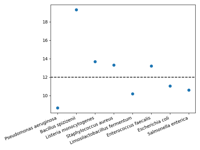
Measured gDNA proportions of a Zymo community

There are some clear discrepancies—Pseudomonas aeruginosa is underreported and Bacillus spizizenii is overreported—but this matches results by e.g. Nicholls et al. (2019).

This short example is intended as a basic demonstration of what's possible in CLIMB-TRE. We're always interested to hear more examples of research questions that CLIMB-TRE can answer, so let us know if you have an example that could be included as a guide for others.